Category Archives: Hobby Coding

Optimising travel time between two locations

AKA Where should my parents-in-law be looking for a house?

With grandchildren numbers rapidly increasing, my wife’s parents have decided to move closer to her and her sister. Houses are uniformly laid out, and roads aren’t always conveniently point-to-point, so this has lead to discussions about what area is suitable for the search

The problem

Given two anchor locations, and a maximum drive time to each, what is the correct region in which my parents-in-law should search for a house.
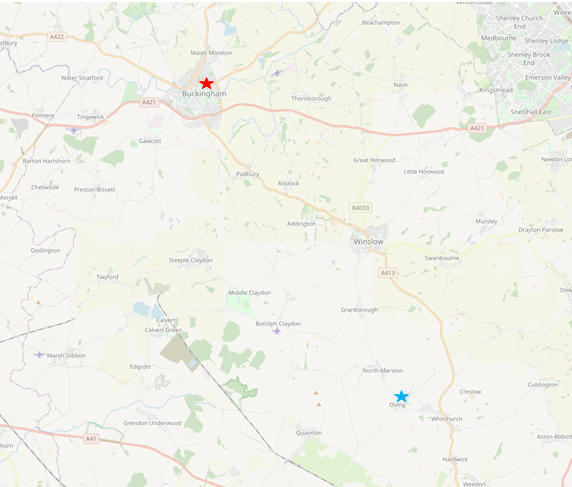
Without being too specific, the red and blue stars are our anchor locations

The solution

After the obligatory googling, I think I’ve found the bones of a solution:

  1. OSMnx – This provides a way to pull data from OpenStreetMap (OSM), including the places, roads and map itself. There are some excellent examples in the git repo, and Geoff Boeing seems to be something of the god in this field
  2. networkx / geopandas – Some useful functions for doing the maths
  3. Folium – For displaying my output

My steps are:

  1. Find 2 OSM nodes to represent my locations
  2. Create a zone around each which represents the distance which can be travelled in a given time
  3. Find the intersection between those two zones
  4. Draw it on a map

1. Finding my points

From the brief time I’ve spent looking at it, OSM seems to work on two main data features, Nodes and Edges. A node is a location of interest on the map, and could be something like a house or shop, or might just be a bit of road. The edges are the (hopefully) legal moves between nodes, and come with some useful metadata like the speed limit on a particular road, and the distance.

For starters I’ll create variables with the rough locations we’re working from

#Setup some locations to work with, my two locations, and a roughly midpoint (might be useful later)
oving=(51.88550,-0.85919)
buckingham=(52.00271, -0.97210)
midPoint=(52.00,-.9)

Then use the OSMnx package to pull back map detail from that

Graw=ox.graph_from_point(mid_point, dist=25000, network_type='drive' )

This takes a few minutes, and populates 4 json files of about 5mb each with lots of location data.

oving_center_node = ox.get_nearest_node(Graw, oving)
buckingham_centre_node = ox.get_nearest_node(Graw, buckingham)
G = ox.project_graph(Graw)

I then use get_nearest_node to give me a known node close to both of my locations, finally ‘projecting’ the data, which as best I understand it, means I’m taking the 3d Lat/Long information, and flattening it to a 2d co-ordinate system from further analysis.

2./3. Create the travel zone around each / find the intersection

This is pulled from another piece of code in the OSMnx git examples, I think the idea is that the ego_graph is able to find all the nodes within a certain distance of the original – in this case the distance is time:

#Use the networkx 'ego_graph' function to gather all my points with a 25 minute drive time
ovingSubgraph       = nx.ego_graph(G, oving_center_node, radius=25, distance='time')
buckinghamSubgraph  = nx.ego_graph(G, buckingham_centre_node, radius=25, distance='time')

#To create the overlap, I found this snippet of code which just removes the nodes only in one side
jointSubgraph=ovingSubgraph.copy()
jointSubgraph.remove_nodes_from(n for n in ovingSubgraph if n not in buckinghamSubgraph)

Then we need to create some polygons which enclose all the nodes:

#For each location, get the points, and then use geopandas to create a polygon which completely encloses them
ovingPoints = [Point((data['lon'], data['lat'])) for node, data in ovingSubgraph.nodes(data=True)]
ovingPoly = gpd.GeoSeries(ovingPoints).unary_union.convex_hull

buckinghamPoints = [Point((data['lon'], data['lat'])) for node, data in buckinghamSubgraph.nodes(data=True)]
buckinghamPoly = gpd.GeoSeries(buckinghamPoints).unary_union.convex_hull

jointPoints = [Point((data['lon'], data['lat'])) for node, data in jointSubgraph.nodes(data=True)]
jointPoly = gpd.GeoSeries(jointPoints).unary_union.convex_hull

4. Draw it on a map

Then, finally plot the 3 regions, and 2 locations on a folium map

#Define some styles for my areas
style1 = {'fillColor': '#228B22', 'color': '#228B22'}
style2 = {'fillColor': '#8B2222', 'color': '#8B2222', 'marker_color' : 'green'}
style3 = {'fillColor': '#22228B', 'color': '#22228B', 'marker_color' : '#22228B'}

#Create a new Foilum map to show my data
mapOutput = folium.Map(location=oving,tiles="openstreetmap",   zoom_start=11)

#Add my polygons
folium.GeoJson(jointPoly, name='Overall', style_function=lambda x:style1).add_to(mapOutput)
folium.GeoJson(ovingPoly, name='Oving', style_function=lambda x:style2).add_to(mapOutput)
folium.GeoJson(Point(oving[1],oving[0]), name='Oving', style_function=lambda x:style2).add_to(mapOutput)
folium.GeoJson(buckinghamPoly, name='Buckingham', style_function=lambda x:style3).add_to(mapOutput)
folium.GeoJson(Point(buckingham[1],buckingham[0]), name='Buckingham', style_function=lambda x:style3).add_to(mapOutput)

#Show the output
mapOutput

and…
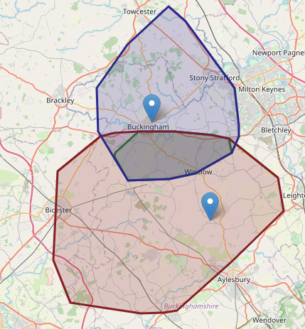
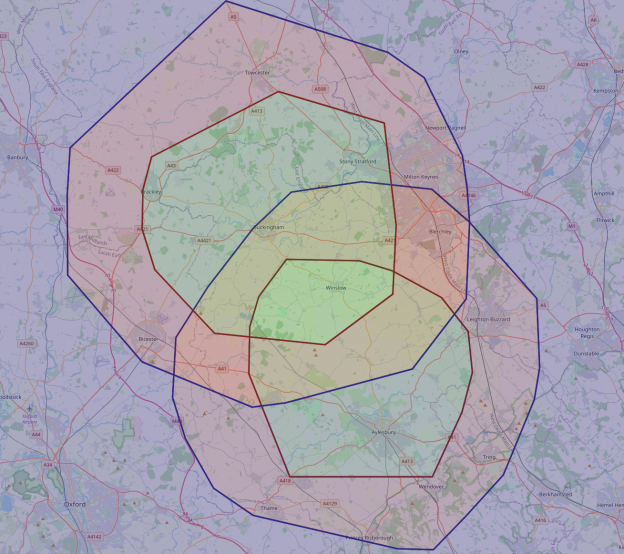
It’s hard to see, but the green polygon is the intersection

Ta-da! we have a working solution.. and much quicker than usual..

But, wait. How is it possible that from the lower location it’s possible to get almost all the way to the upper location, but not vice-versa?

Also, that middle ‘green’ section (which is a bit hard to see) doesn’t entirely cover the intersection.

What went wrong

I think 2 things are broken:

  1. The ‘ego graph’ function isn’t correctly returning the nodes with a travel time
  2. The generated polygons are optimised to enclose regions in a way which could under play the intersection

I think #1 is the result of trying to pull apart another solution, the ego graph is obviously unable to perform the analysis I want to do. I think it’s doing a simpler calculation of all the nodes within 25 connections of the original. The lower point is in a village, and so will need to travel further to reach 25.

#2 is probably more of a finessing problem.

Improving the solution

I need to find a way to identify all the points within a certain drive time of the starting point. Luckily OSMnx has some extra features to help with that.

ox.add_edge_speeds(Graw)
ox.add_edge_travel_times(Graw)

This should add some extra data to each edge to help compute the travel time between each

#Get the shortest path
shortest_path = ox.shortest_path(Graw, oving_center_node, buckingham_centre_node, weight='length')
#Plot it on a map
ox.plot_route_folium(Graw, shortest_path)
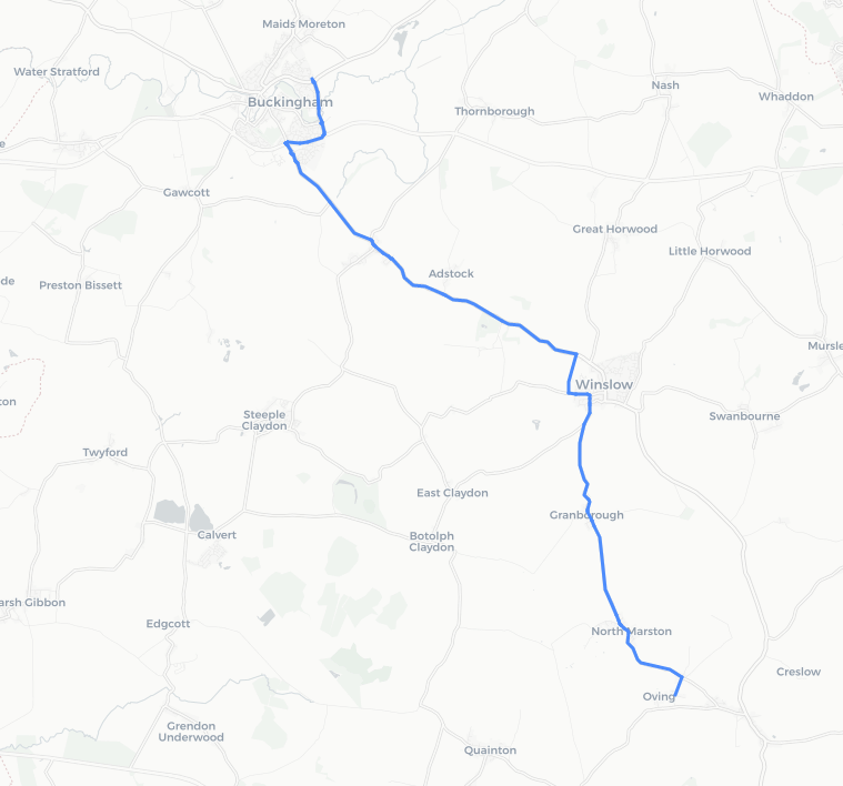
looks ok, but that route definitely takes in a bridleway.. one for another time!
#Get the shortest path
shortest_path_time = nx.shortest_path_length(Graw, oving_center_node, buckingham_centre_node, weight='length')
print(shortest_path_time)

18955.. Presumably metres? a quick check of google maps suggests it’s probably true. so 18km.

#Get the shortest path
shortest_path_time = nx.shortest_path_length(Graw, oving_center_node, buckingham_centre_node, weight='travel_time')
print(shortest_path_time)

Weighting it by travel time returns 1040. If that’s in seconds, the trip is about 17 minutes.

I think the journey actually takes more like 25, even if we ignore traffic, I don’t think it’s correctly pricing in the time to accelerate, and things like traffic. But anyway, we have a way forward.

The ‘not very optimal, but will probably work’ solution goes like: Loop through all the nodes in the overall map, check the travel time, keep them (if it’s below the threshold)

ovingPoints = [Point((data['lon'], data['lat'])) for node, data in G.nodes(data=True) if nx.shortest_path_length(Graw, oving_center_node, node, weight='travel_time')<25*60]

So I ran that, and it took ages. There are 39k nodes in that section of the map. There’s going to be a huge amount of recursion going on too, so not very efficient. I need a different approach

Intermission: How *does* google calculate drive time?

While playing around with this I checked the drive time to a few other places and it seems to always be very fast compared to google
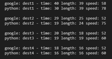
4 random destinations, showing the difference between what google says, and what I’ve got from the code

The distances are thereabouts, the time is the problem. Digging in a bit more, the time calculation is literally adding the time to traverse each edge, assuming you can travel at the maximum speed possible on that bit of road. Not hugely realistic.
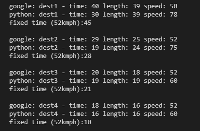
The ‘fixed’ time is the time it would take assuming you travel at 52kmph the whole way

I’m not really here to replicate google, at very least I’d just hook into the API, but that’s for another day. For now, I’ll just recalculate my speed for any journey which has an average above 52. This will reduce the likelihood of very distant nodes making it into the allowed zone, which is what I’m wanting anyway.

Back to the problem

My latest issue is that I can’t check every node in the graph in a reasonable amount of time. So the next idea is to reduce the scope of the checking. I don’t need to check every node, but I want to make sure I cover a reasonable area
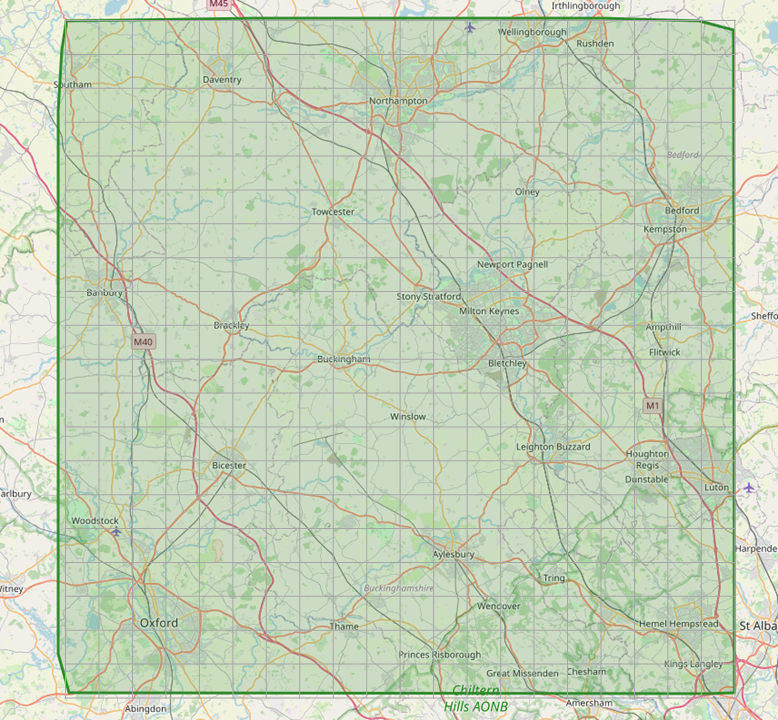
The map area in green, with a hypothetical grid over the top

If I imagine a grid over the whole map area, I can loop through regular points on that grid, get a node near the point, and then check the distance from my starting points to that node

First, get the bounding box of the map area:

north, south, east, west = ox.utils_geo.bbox_from_point(midPoint, dist=35000)
north=math.ceil(north*100)/100
south=math.floor(south*100)/100
east=math.ceil(east*100)/100
west=math.floor(west*100)/100
print(north, south, east, west)

Then define 400 boxes and calculate the Lat/Lon points for each

steps=20

grid=[]
for i in range(steps+1):
    lat=south+(i*round(north-south,2)/steps)
    for j in range(steps+1):
        lon=west+(j*round(east-west,2)/steps)
        node=ox.nearest_nodes(Graw, lon, lat)
        grid.append(node)

Now, loop through each point, find the nearest node, and calculate the time to get to it

ovingPoints=[]

for node in grid:
    try: #This is to capture the cases where the selected node has no path back to the origin.. I'm not bothered about these
        shortest_path = nx.shortest_path(Graw, oving_center_node, node, weight='travel_time')
        length=int(sum(ox.utils_graph.get_route_edge_attributes(Graw, shortest_path, 'length')))/1000 #in KM
        time=int(sum(ox.utils_graph.get_route_edge_attributes(Graw, shortest_path, 'travel_time')))/60 #in mins
        speed = (length)/(time/60) #speed in kmph
        if speed > 52: #If the hypothetical speed is ever greater than 52kmph, reduce it to that number
            time = (length/52)*60
        newPoint=Point((Graw.nodes[node]['x'],Graw.nodes[node]['y']))
        ovingPoints.append((newPoint, time, length))
    except: 
        pass
        

Finally build some polygons which encompass reasonable travel times, less than 20 mins, 20-30 and 30+

ovingPointsLow = [point for point, time, length in ovingPoints if time < 20]
ovingPolyLow = gpd.GeoSeries(ovingPointsLow).unary_union.convex_hull

ovingPointsMid = [point for point, time, length in ovingPoints if (time >= 20 and time <30)]
ovingPolyMid = gpd.GeoSeries(ovingPointsMid).unary_union.convex_hull

ovingPointsHi = [point for point, time, length in ovingPoints if time >=30]
ovingPolyHi = gpd.GeoSeries(ovingPointsHi).unary_union.convex_hull
ovingPolyHi=ovingPolyHi-ovingPolyMid
ovingPolyMid=ovingPolyMid-ovingPolyLow

And plot the result on a map:

That’s better!

I’m happier with both the extent of the regions (I think that’s a reasonable distance to travel in the time – ignoring rush-hour around Aylesbury)

The regions are also much more circular, and critically, overlap.

Now, a bit more polygon maths and we can calculate the definitive areas of interest

buckinghamPolyLowMid = buckinghamPolyMid.union(buckinghamPolyLow)
ovingPolyLowMid = ovingPolyMid.union(ovingPolyLow)
jointPolyLow = buckinghamPolyLow.intersection(ovingPolyLow)
jointPolyLowMid=buckinghamPolyLowMid.intersection(ovingPolyLowMid)
#Create a new Foilum map to show my data
mapOutput = folium.Map(location=oving,tiles="openstreetmap",   zoom_start=13)

#Add my polygons
folium.GeoJson(jointPolyLow, name='Low', style_function=lambda x:style1).add_to(mapOutput)
folium.GeoJson(jointPolyLowMid, name='Low', style_function=lambda x:style2).add_to(mapOutput)

#Show the output
mapOutput
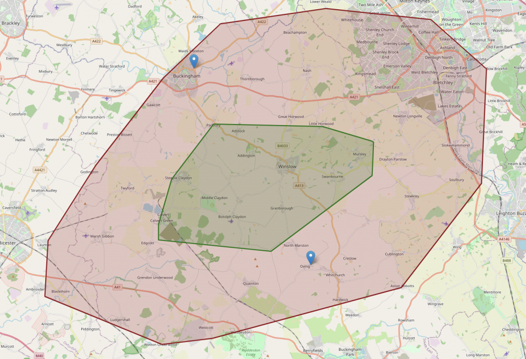
Green is within 20 mins of both, red is 20-30 mins from both

Ta-da!

I’ll let them know.
Using Object Detection to get an edge in TFT [pt2]

<see part one for the whole story>

While mulling my options for the next steps on this project, I got some feedback

i think the backgrounds will be your biggest issue…that followed by the healthbars / items equipped…trying to normalise for that will probably help a lot ?

Tom Cronin – via Linkedin

Which completely changed my view on the problem.

Firstly, I’d thought the background were *helpful* – the high contrast with the characters, and then the different backgrounds that players use to provide variety. A problem I’d not considered is how much extra complexity they add into the image, and how much more training might be needed to overcome that.

Secondly, I’d been thinking my task was to collect and annotate as many images as possible.

I’ve been doing it wrong.

The (new) approach

I can easily ‘cut’ the characters out from their backgrounds

Mad as it sounds, I did this in Powerpoint. The ‘background eraser’ tool is the quickest and most accurate I’ve found.

But then the problem is that I don’t want the computer thinking a solid white rectangle is anything meaningful to the character. So what if I take the cut out, and make some new backgrounds to put it on. Then I’m killing two birds with one stone:

  1. I can create any background I like; colours, shapes, pigeons.. and:
  2. I can create LOTs of them

So rather than screenshotting and annotating, my new approach is:

  1. Cut out a lot of character images (this is tedious, but once it’s done, it’s done forever.. or until the next patch)
  2. Create some random backgrounds
  3. Stick the characters over the new backgrounds
  4. Auto-generate the boundaries I had to draw manually last time

Step 0

There’s always a step 0.

Up to this point, I’ve been hacking about, every step is manual, most of them are ‘found’ by clicking up and down through the terminal window.
I’ve now written a single script which automates:

  1. Clear output folders
  2. Create images (and the annotation file)
  3. Create test/train split
  4. Create TFRecord files

(at some point I’ll automate the run too, but this at least gives me a start)

Step 1 – Cut out a lot of images

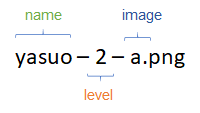
This isn’t very interesting, but I noticed through the process that the characters move about a bit. Just small animation loops for most, but some even flip sides. On that basis, I’ve used a naming convention for the files which allows me to have multiple copies

Each character has 3 levels, which are gained as you get more of them (3 of the same magically transforms into level 2, and 3 level 2s become a level 3). Power increases quite significantly with level.

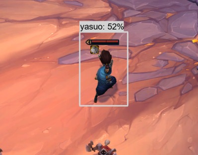
Here are Yasuo A and B – same colours, but different pose

I keep the first two sections as the class I’m trying to predict, but ignore the suffix.

Step 2 – Create some random backgrounds

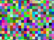
Thinking about the backgrounds, I initially went with 2 options – a blurry ‘noise’ of colour, and a single flat colour. The overall intent is that the computer loses the overall background as it learns, and just focuses on the character.

some pixely noise, I’ll assume you can imagine a flat colour

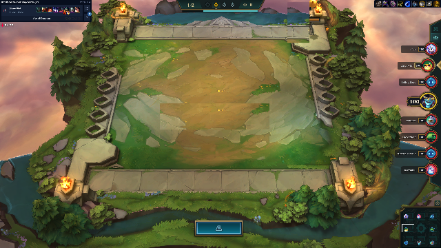
I noticed in early testing that computer was labelling some odd things like parts of my desktop background, while failing on actual screenshots from the game. I decided to add in a handful of random backgrounds from the game (with any characters removed) to give some realism to the sample

one of 8 random backgrounds

Step 3 – Stick the characters over the new backgrounds

I then load a random character image (so random character, level and pose) from my input folder, and add it to the image. I’ve also added a chance for the image to be resized up or down a little before it’s added – this is to cover the slight perspective the game adds, where characters in the background are smaller.

I repeat the loop 20 times for each image, and save it down with the xml

Some of them are in unlikely places, but that should matter less than having accurate backgrounds in there
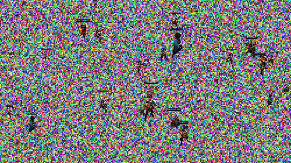
AVERT YOUR EYES.. this looks horrible, but should help the computer realise the background isn’t important

Step 4 – Auto-generate the boundaries I had to draw manually last time

I was very pleased when this worked.

The most tedious task of the original attempt is now gloriously automated. Each character image reports it’s location and size, and is added in to the correct xml format.

I can now create hundreds, or thousands of files to use as inputs!

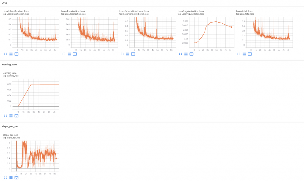
So, what does this do to the graph?!

(I should note, with this change I’ve also tweaked some parameter files. I’m not entirely sure of the sensitivity, but each run now uses multiple images. This might only have the effect of doubling the time per step, and halving the number of steps needed. Idk)

Well, a few things look different:

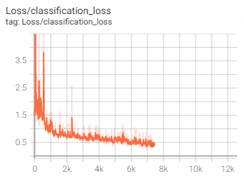
My loss (which I’m assuming is the equivalent of 1/accuracy) behaves much more at the start, and quickly follows a steady curve down.

The time/step is *horrendous* for the first 1k steps. The run above was over 6 hours.

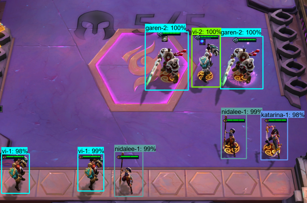
tl;dr – did it work?!

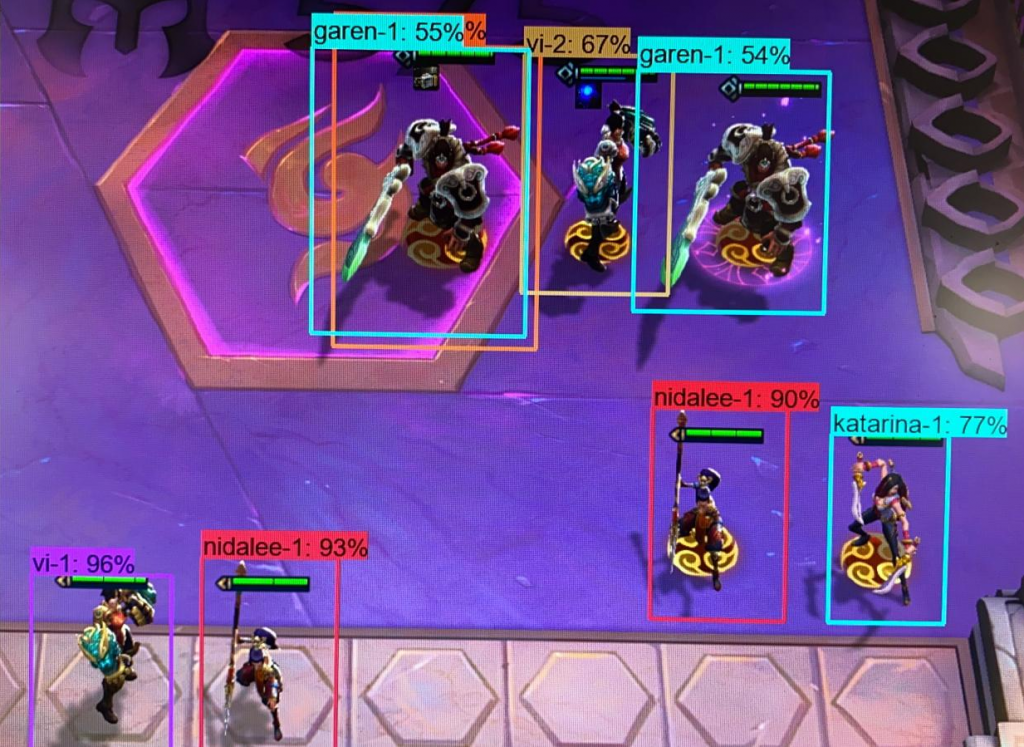
Assuming no prior knowledge, I can tall you that every guess is correct.

Just a bit.

This isn’t just better, it’s remarkable. Every character is guessed, and the strength of the prediction is almost 100% each time. It’s spotted the difference between the Level 1 & 2 Vi, and even handled the inclusion of an ‘item’ (the blue sparkly thing below her green health-bar)

Appendix

The early run (pre the inclusion of backgrounds) did better than before, but still lacked the high detection numbers of the most recent model

This is based on the same character images, but the model also has ‘real’ backgrounds to sample too

It’s especially confused when the background gets more complex, of there’s overlap between the characters.

I’ve also started looking at running this on screen capture, rather than just flat images. I think the hackiness of the code is probably hampering performance, but I’m also going to look at whether some other models might be more performant – e.g. those designed for mobile.

Even with the low frame-rate, I’m delighted with this!

Using Object Detection to get an edge in TFT [pt1]

Teamfight Tactics (TFT) is an auto-battler game in the League of Legends universe. Success depends on luck, strategy, and keeping an eye on what your opponents are doing. I wonder if I can use the supreme power of TensorFlow to help me do the last bit?

TFT best comps: how to make unbeatable teams | Rock Paper Shotgun
I won’t bother explaining the concept, for now, just that it’s useful to know what all the things on the screen above are

The problem

Given a screenful of information, can I use object detection & classification to give me an automated overview?

What I’ve learned about machine learning

I usually write these posts as I’m going, so the experience is captured and the narrative flows (hopefully) nicely. But with this bit of ‘fun’ I’ve learned two hard facts

  1. Python, and it’s ecosystem of hacked together packages, is an unforgiving nightmare. The process goes like this: a) install package, b) run snippet of code, c) try to debug code, d) find nothing on google, keep trying, e) eventually find reference to bug reported in package version x f) install different version [return to b]. It’s quite common to find that things stopped being supported, or that ‘no-one uses anything after 1.2.1, because it’s too buggy’. It’s also quite common to only make progress via gossip and rumour.
  2. The whole open source ML world is still very close to research. It’s no wonder Google is pushing pre-packaged solutions via GCP, getting something to work on your own PC is hard work, and the steps involved are necessarily complicated (this *is* brain surgery.. kinda)

But I’ve also found that I, a mere mortal, can get a basic object detection model working on my home PC!

The Approach

This is very much a v0.1 – I want to eventually do some fancy things, but first I want to get something basic to work, end to end.

The very basic steps in image detection & classification. The black box is doing most of the interesting stuff

Here are the steps:

  1. My problem – I have an image containing some (different) characters which I want to train the computer to be able to recognise in future images
  2. I need to get a lot of different images, and annotate them with the characters
  3. I feed those images and the annotations into a magic box
  4. The magic box can then (try to) recognise those same characters in new images

One of the first things I’ve realised is that this is actually two different problems. First, identify a thing, then try to recognise the thing

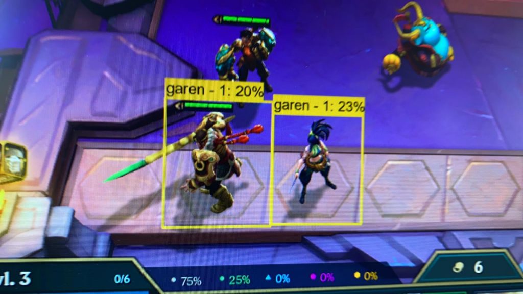
One of these is Garen, the other is Akali. The confidence in the guess is misplaced.

In this early run, which I did mainly to test the pipework, the algorithm detects that the 2 characters in the foreground are present, but incorrectly labels one of them. In it’s defence, it’s not confident in EITHER.

So, to be clear, it’s not enough that I can teach it to recognise ‘character-like’ things, it also has to be able to tell them apart.

Step 1: Getting Tensorflow installed

I’ve had my python whinge, so this is all business. I tried 3 approaches:

  1. Install a docker image
  2. Run on a (free) google colab cloud machine
  3. Install it locally

In the end I went with 3. I don’t really understand docker enough to work out if it’s broken, or I’m not doing it right. And I like the idea of running it locally so I understand more about the moving parts.

I followed several deeply flawed guides, before finding this one (Installation — TensorFlow 2 Object Detection API tutorial documentation) which was only a bit broken towards the end. What I liked about this was how clear each step was, and upto a certain stage, everything just worked.

Step 2: Getting some training data

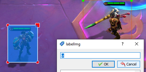
I need to gather enough images to feed into the model to train it, which I’m doing by taking screenshots in game, and annotating them with a tool called labelImg

This is the less glamourous bit of machine learning, drawing boxes around everything of interest, and labelling them

I’m not sure how many images I need, but I’m going to assume it’s a lot. There are 59 characters in the game at the moment, and each of those has 3 different ‘levels’. There are also other things I’d like to spot too, but for now, I’ll stick with the characters.

I’ve got about 90 images, taken from a number of different games. The characters can move around, and there are different backgrounds depending on the player, so there should be a reasonable amount of information available. There can also be the same character multiple times on each screenshot.

I started out labelling the characters as name – level (e.g. garen – 2), which is ultimately where I want to be, but increasing the number of things I want to spot, while keeping the training data fixed means some characters have few (or no) observations.

Step 3: Running the model

I’m not going to describe the process in too much detail, I’ve heavily borrowed from the guide linked earlier, the rough outline of steps is as follows:

  1. Partition the data into train & test (I’ve chosen to put 25% of my images aside for testing)
  2. Build some important files for the process – one is just a list of all the things I want to classify, the other (I think) contains data about the boxes I’ve drawn around the images.
  3. Train the model – this seems to take AGES, even when run on the GPU.. more about this later
  4. Export the model
  5. Import the model and run it against some images

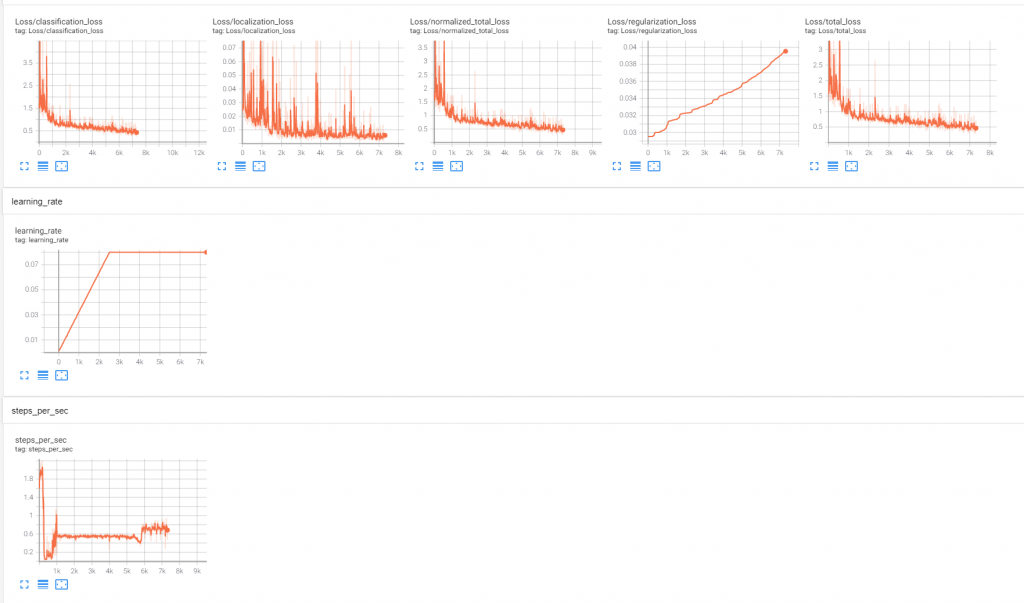
During the training, I can monitor progress via ‘Tensorboard’, which looks a bit like this:

I’m still figuring out what the significance of each of these measures is, but generally I think I want loss to decrease, and certainly to be well below 1.

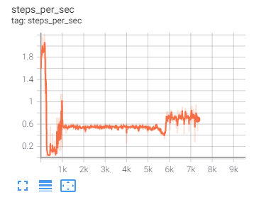
An interesting thing I noticed was that the processing speed seems to vary a lot during run, and particularly drops off a cliff between steps 200 and 300

I’m not sure why this is happening, but it’s happened on a couple of runs, and when the speed increases again at around step 600, the loss becomes much less noisy

I should get a more zoomed in chart to illustrate, but you can see that the huge spikes disappear about half-way between 0 and 1k steps

There seems to be a gradual improvement across 1k+ steps, but I’m not sure if I should be running this for 5k or 50k. I also suspect that my very small number of training images means that the improvement will turn into overfitting quite quickly.

Step 4a: The first attempt

I was so surprised the first attempt even worked, that I didn’t bother to save any screenshots of the progress, only the one image I gleefully sent on whatsapp

At this stage, I realised that getting this to work well would be more complicated, so I reduced the complexity of the problem by ignoring the character’s level

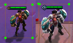
Vi level 1, left, Vi level 2, right

The characters do change appearance as they level up, but they’re similar enough that I think it’s better to build the model on fewer, more general cases.

Step 4b: The outcome

(this is correct)

Success! A box, drawn correctly, and a name guessed which is correct!

hmm.. maybe a bit less correct

Ok, so that first one might be a bit too good to be true, but I’m really happy with the results overall. Most of the characters are predicted correctly, and I can see where it might be getting thrown by some of the graphical similarities

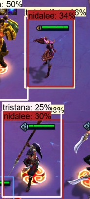
Here, for example, the bottom character is correctly labeled as Nidalee, but the one above (Shyvana) has a very similar pose, so I can imagine how the mistake was made

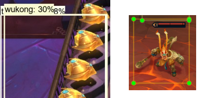
And here, the golden objects on the side of the screen could be mistaken for Wukong.. if you squint.. a lot

Next steps

I’m really pleased with the results from just a few hours of tinkering, so I’m going to keep going and see if I can improve the model, next steps:

  1. More training data
  2. Try modifying the existing images (e.g. removing colour) to speed up processing
  3. Look at some different model types
  4. Try to get this working in real-time

Most of the imagery on this page is of characters who belong to Riot, who make awesome games

<See part 2 here>

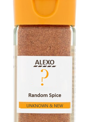
Random Spice

I’m a bit bored of the herbs and spices in my cupboard, I wonder if I can make a better one?

Wouldn’t it be exciting?

The Problem

I want to create a new herb or spice, it needs a name and a description.

I want to ingest (haha) all the herbs and spices in my cupboard (the ‘legacy’ group) and then use that to generate new ones.

The Approach

I’ll start with a simple N-gram text generator. This works by ingesting a corpus of existing valid input, and ‘learning’ how to make valid outputs by using combinations it knows, for example:

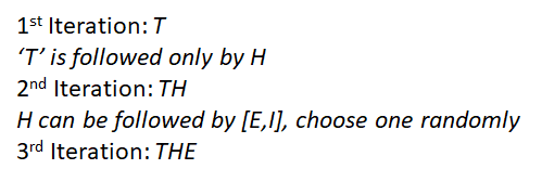
Lets train on the valid words [“THE”, “THIS”], and assume we only look at 1-grams (1 letter at a time). T is the first letter, T is always followed by H, H can be followed by E or I, I is always followed by S. This gives the program the rules it can use to make ‘new’ words. An iterative loop can be used, for example:

This is a pretty straightforward example

This recreates the word ‘THE’ by randomly choosing next letters which it has seen following the last letter. The possibilities get more complex with a greater selection of words, as we’ll see.

The steps for the problem are

  1. Generate some new names based on the legacy group
  2. Generate a description
  3. Look at the optimal parameters

0. Make an N-gram function

(I assume this already exists, but I’m not going to learn by pip installing things)

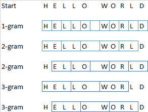
I’ll take N-gram to refer to the cutting up of parts of my text input into groups of N-size.

Here are some N-gram breakdowns of the initial phrase

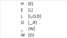
Here I’ve done it by character, with increasing values of N. If I take the simplest 1-gram, I can make a list of which letters follow others:

H only has one option (E), but L could be one of 3 options (L,O,D). _ is a space

I’ll get that working in Python, but I want the flexibility of selecting a value of N, and also the option to have separate words treated as distinct pieces of information (in the HELLO WORLD example, O wouldn’t be followed by _ and _ wouldn’t be followed by W)

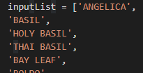
inputList = ["HELLO", "WORLD"]
#Set value of N
N=2

#Get all the N grams (as strings, for N>1)
nGrams = [["".join(input[n:n+N]) for n in range(len(input)-N+1)] for input in inputList]
#I think it's to n+N+1 rather than n+N because the range isn't inclusive.. I should check that

#Within each list of n-grams, return it and the next character into a list
links = [[[subarr[i], subarr[i+1][N-1]] for i in range(len(subarr)-1)] for subarr in nGrams]

#Flatten the list of lists
flatLinks = [subLink for link in links for subLink in link]

print(flatLinks)

This is for N=2. You’ll see the initial 2-gram is followed by the single character which would come next. If this was going to be much longer or more complex, I’d find a more efficient structure.

1. Generate a new name

In order to make this I’ll need a starting list of names. I’ve borrowed this from Wikipedia.

That’s 200% more basil than I was aware of

The same code will now generate a much longer list of the different N-gram associations

You can still make out the individual legacy names

The process is now to create my new name using a loop, to start I’ll randomly pick one of my 2-grams to use as a seed, then:

  1. Look-up every instance of the last 2-gram in the name
  2. Randomly choose one of the associated next letters
  3. Add this to the name
import random
output=""
lastbit = random.choice(flatLinks)[0]

output=output+lastbit

for i in range(10):
    print("lastbit")
    print(lastbit)
    matchList=[n for n in flatLinks if n[0]==lastbit]
    print("matchList")
    print(matchList)
    lastbit=random.choice(matchList)
    print("lastbit[1]")
    print(lastbit[1])
    output=output+""+lastbit[1]
    print("output")
    print(output)
    lastbit="".join(output[-N:])
print(output)
I assume this is how my cats think, just replace letters with ‘EAT’, ‘HUNT’, ‘SLEEP’

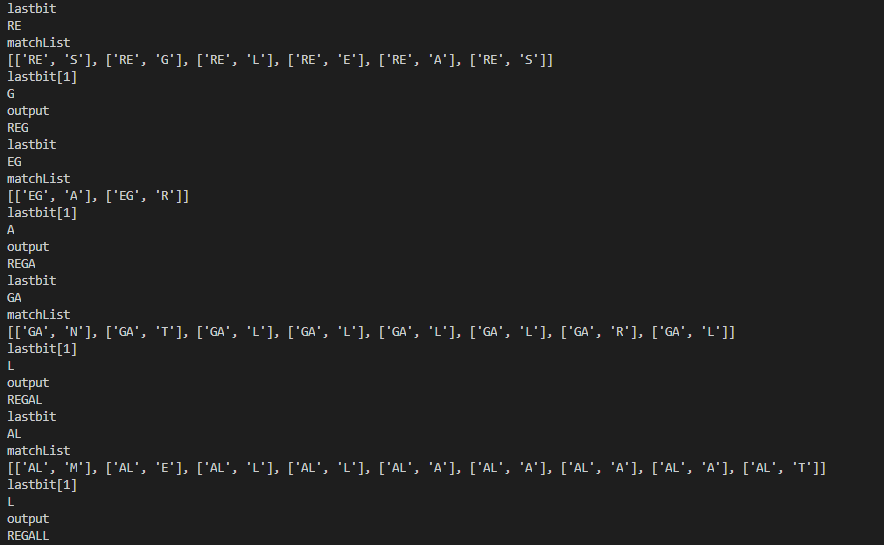
And here’s an example. The code has started randomly with the letters RE. That gives options of S, G, L, E, A and S. It randomly chooses G, adds it to the output name, and then recalculates the last 2 letters of the name. The loop repeats for 10 letters, and gives us our new name:

I’m pronouncing it Re-galable

Regallaball! A brand new spice (or herb?) and I didn’t even have to leave the house!

But what’s it like?

2. Generate a description

My existing n-gram generator will almost work for this, but I need to make a tweak. I’m going to be using whole words, rather than individual letters to build up the description, so I need to add a split() in to the initial n-gram list comprehension:

nGrams = [["".join(input[n:n+N]) for n in range(len(input)-N+1)] for input in inputList]
#becomes
nGrams = [[" ".join(input.split()[n:n+N]) for n in range(len(input.split())-N+1)] for input in inputPhraseList]
#I've also changed the name of the input variable

My input now needs to be some relevant descriptions of the legacy group, the wikipedia descriptions are a bit formal (and specific) and I don’t think they’ll lend themselves to generating meaningful descriptions, so after a bit of googling I found this website with some which I’ll borrow blog.mybalancemeals.com

They aren’t perfect, especially when they’re self referential, but I’ll use this for starters. Just a small tweak to the output generation code (to put spaces between the words) and we’re ready to generate!

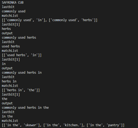
Ah. I’ve got a problem. This could have come up in the name generator, but using combinations of letters made it less likely. The problem is that the code is asking for a combination of lookup words which doesn’t exist. The debug trace show us why:

No problems yet

My new creation is called ‘Safronka Cub’, and as the description builds, it starts out well. Safronka Cubs are commonly used herbs..

IndexError: list index out of range

But once we hit the end of a sentence, where there is no viable continuation of the loop, as the list of matches is empty. Let’s code around that:

for i in range(60):
    print("lastbit")
    print(lastbit)
    matchList=[n for n in flatLinks if n[0]==lastbit]
    if (len(matchList)>0): #protect against lookup errors
        #print("matchList")
        #print(matchList)
        lastbit=random.choice(matchList)
        #print("lastbit[1]")
        #print(lastbit[1])
        output=output+" "+lastbit[1]
        #print("output")
        #print(output)
        lastbit=" ".join(output.split()[-N:])
print(output)
Side effect of this project is a lot of snacking

Which, critically, is not in my input text (well, mostly)

Probably a bit too close to be genuinely novel

3. Look at the parameters

The key parameter in my N-grams is the N. Longer and it will produce more realistic things, but it will do that by copying more and more of the original. Shorter and the output will be novel, but garbage. With a bit of refactorising, I can generate a series of different names, varying the N parameter.

N=1N=2N=3N=4N=5
IARYMORREDHERY SEEDOARBEANCUMINHERVIL
AZETAF PAJIALABASMARDAMPEPPERIFERILSHOLTZIA CILIAYNGIUM FOETIDA
TOLILERRDIPEEDOATIDUMINERICELYTHRUMFERIA GALANGAL
LAVAMOLEMEKPEREEDOARONERICELERYNGIURDAMOMMUSTARD
IGELITSEEDOANDER SEEDEPPERCORNPEPPERCORN
NDILATITZEML ANISELEMPFAMPHORSER GALSTARDIMNOPHILA AROMA
NGERANTIGEGRY LIA ANS OERILLAPEPPERCORNOLY BASIL
PABAREBRISSTSERUEROLIVIAN PEPPUZU (ZESTEMON MYRTLE
IARASAN AGALIANDERUVIETNNELJIMBUIGELLA
SASSETUMALEIANGIND DILITIDUMLEAFARADISH
Blue are those which my brain sees as possible genuine names, red are those which are copies, or almost copies of the genuine once

Length aside, the trend seems pretty clear, as you increase N, the number of valid responses increases, but above 4, it’s dominated by copies of the original names.

The number of inputs is quite small, and the nature of the inputs means that beyond 3, there is almost no randomness when the name is built.

Here’s the same thing for the descriptions (red text is a straight copy of the original).

N=1 (gibberish)

  • as strong pine flavour you can be consumed fresh, dried, and Jamaican jerk chicken.
  • number of cooking, pairing often compliments the delicate leaves mostly complement fish tacos to the flavourful power duo in curry powder mostly consists of dill here, including bistromd’s mini pies using simple ingredients to preserve the strong and avocado!

N=2

  • salads, baked potatoes, creamy potato salad, deviled eggs, and can be added into butters, vinegars, and sauces for added flavor depth.
  • a flowering plant with the seeds added to the whole garlic head in these roasted garlic velouté sauce to the taste of soup, others who enjoy it describe it as a mild tasting parsley with a number of cuisines. the nutty flavor is widely used in soups, stews, and roasted dishes. in addition to rosemary in the pantry and offers an accelerated

N=3

  • coming from a hot chili pepper, cayenne pepper offers spice to a number of dips, complement various casseroles, along with these other 25 ways to use parsley.
  • the strong pine flavor of rosemary pairs well with various flavors, including this chocolate mint smoothie and fizzy blueberry mint drink. along with its value in numerous recipes, the herb also provides an extensive number of health benefits.

N=4

  • are commonly used in soups, stews, and for pickling hence “dill pickles.” find eight flavorful recipes to use a bunch of dill here, including grilled carrots with lemon and dill, zucchini with yogurt-dill sauce, and golden quinoa salad with lemon, dill, and avocado!
  • the end of cooking, pairing well with mexican dishes, fish, or soups and salads.

N=5 (straight copy)

  • a spice described as strong and pungent, with light notes of lemon and mint. for the freshest flavour, purchase whole cardamom pods over ground to preserve the natural essential oils. find over 30 cardamom recipes here.
  • note to a number of soups, stews, and roasted dishes. in addition to rosemary in the skewer recipe provided above, thyme further compliments the meat.

Again, beyond N=3, the algorithm is locked to the original source text, even at <=3, it’s typically returning odd chunks of text.

4. Refining the descriptions

Although I’m happy with the code, the descriptions I’ve scraped aren’t working well. I’ve found another source, which is a bit more focussed on the flavour. I’ve also tweaked the definitions to remove any mention of the original name. Finally I’ve tweaked each to start with ‘This..’ so I can be sure that my descriptions start at the beginning of the sentence.

The code will also flag any iterations which yield results which are identical, or substrings of the inputs.. and here’s what I get (corrected here for British spelling).

5. The result

Uzaziliata
This can be sprinkled onto or into sauces, pastas, and other dishes to add a nutty, cheesy, savory flavor.

Avender Seed
This herb smells like maple syrup while cooking, it has a mild woodsy flavor. can be used to add a nutty, cheesy, savory flavor.

Tonka Berroot
This is Sometimes used more for its yellow colour than its flavour, it has a mild woodsy flavour. Can be used in both sweet baked goods and to add depth to savoury dishes. (it’s also almost a google-whack!)

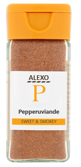
Pepperuviande
This Adds sweet smokiness to dishes, as well as grilled meats.

Any resemblance to spices living or dead..

Much better, right?

Here’s the code https://github.com/alexchatwin/spiceGenerator

Charting my Smart Heating system

Background

When the baby was born, I championed the installation of a new ‘Smart’ heating system. Our house is very much one that jack built, and the temperature can vary widely between rooms based on things like wall/window quality, wind, sunlight. It’s very useful to be able to control the radiators in each room based on what the room needs, rather than centrally applying a schedule, and trying to tweak the radiators.

I opted for Tado, based on a few factors. I’m not 100% sure it was the best option, but it’s really improved the balance of heating across the house. One of the reasons I chose Tado was the ability to query and make changes via the API.

The problem

“Won’t the baby get cold?”

It’s a throwback to an old technology, those of us born before digital stuff became so cheap are very used to anachronisms like turning the heating up higher to ‘make it warm up faster’. I’m keen to find a way to use the API to demonstrate to my wife that the baby’s room is

  1. The right temperature
  2. Below the heating capability of the system (i.e. if we had a blizzard, the radiator could call on extra heat to cope)
  3. There’s no need to change the settings

The steps

  1. Get data from the Tado API
  2. Format it into something useful
  3. Decide how to visualise it

1. Get data from the Tado API

I’ve done some messing with Tado before, and I made another post about automating the getting of a bearer token for access, based on some environment variables with my credentials. Given that, and the limited knowledge of the APIs contents, gleened from much googling, I created the following methods:

    def getTadoHome(): #From our auth credentials, return the homeId 
        response = requests.get('https://my.tado.com/api/v1/me', headers={'Authorization': 'Bearer'+auth.returnTadoToken()})
        return response.json()['homeId']

    def getTadoResponse(zoneId, date): #Return a response object for the given zone, on the given day
        endPoint='https://my.tado.com/api/v2/homes/'+str(getTadoHome())+'/zones/'+str(zoneId)+'/dayReport?date='+str(date)
        response = requests.get(endPoint, headers={'Authorization': 'Bearer '+auth.returnTadoToken()})
        return response

    def getTadoRoomTempReport(response):
        response=json_normalize(response.json()['measuredData']['insideTemperature']['dataPoints'])
        roomTemp_df=pd.DataFrame(response)
        roomTemp_df['timestamp']=pd.to_datetime(response.timestamp, format='%Y-%m-%d %H:%M:%S.%f')
        return roomTemp_df

#shortened

Tado lumps up a bunch of the data you need to review a large chunk of time into a single ‘dayReport’ – a monstrous object which is really unpleasant to parse. I’ve solved the problem bluntly by pulling a single dayReport and then passing it to other functions which cut it up.

I’ve also take the time to cut out and rename columns to make them a bit easier to use later. A frustration is how verbose this syntax is in python. A simple rename goes from

select roomheating.from_ts as from

to (what feels like an unecessary):

roomHeating_df.rename(columns={'from': 'from_ts'}, inplace=True)

It’s made more frustrating by having to separate out my renames from my dropping of columns – which can’t be a simple ‘keep’ like in SQL or SAS

2. Format it into something useful

My lack of familiarity with Python, and Pandas specifically might be showing here. I’ve got some datasets which are roughly indexed on time, and I want to join them. I could reflex some SQL to solve this.. but that won’t teach me anything.. so the first step is to think about the data I’m going to merge

again, this kind of merge in SQL would be easy, but after some googling I’ve got an equivalent Pandas syntax:

df_merge=pd.merge_asof(roomTemp_df,roomHeating_df, left_on="timestamp", right_on="from_ts", direction="backward")

Which produces what I’m after, well sort of

Again, I don’t like how verbose this is making a simple join – I’m going to have to do this a few times for each join I want, and it *feels* clunky. I also dislike how it’s keeping all my columns, especially the horrible datatimes

3. Deciding how to visualise it

3a. A rant

Packages are a necessary evil of an open source language which boasts the flexibility of Python, but it comes at a cost. There are a colossal number of ways to do anything, and because they’re all optimised for slightly different end goals, they all work a bit differently.

I’m trying to draw a graph. I want to do this as easily as possible but I’ve no idea where to start, or at least where *best* to start.

3b. Getting on with it

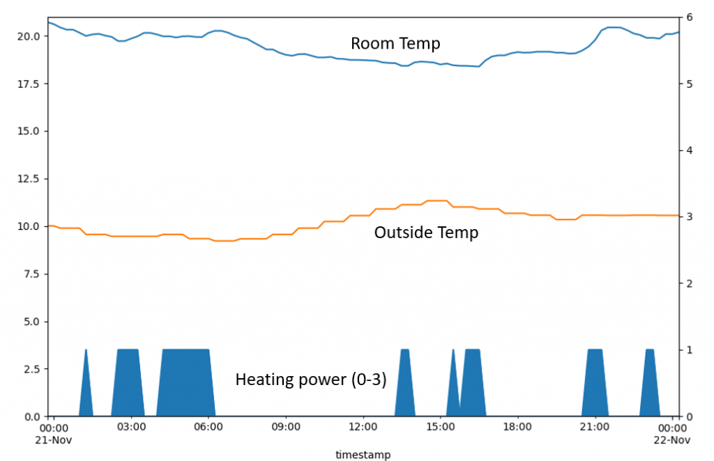
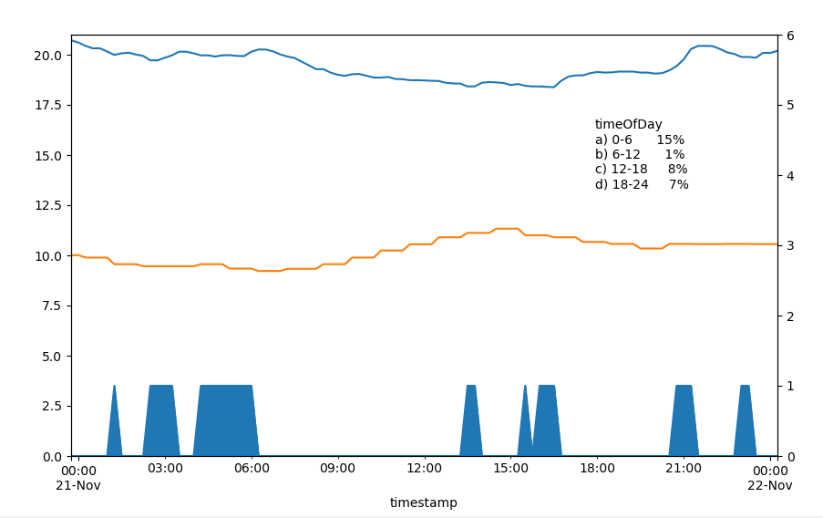
Ok, back to the task. I’ve gone with Matplotlib, largely thanks to google. Here’s a basic plot showing the room temp, external temp, and a measure of the amount of heating power being supplied to the room

This is pretty good – I’ve got the data for a single day, and by converting the heating power value to an integer (from None, Low, Med, High), I can make it clear what’s happening.

First thing to notice is how little heating power is needed to maintain a fairly even room temperature. There’s definitely more capacity in the system. If the system was running at full power all day it would give an average power of 3. With a bit of work to split up the day into 4 time zones:

I can see the amount of power being used to keep the room warm – midnight to 6 am is the worst spot, where we’re using 15% of maximum heating we could give.

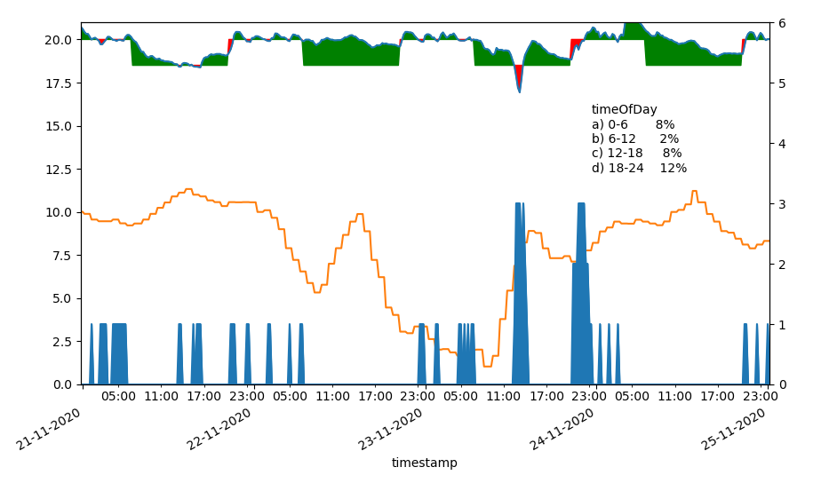
The top line is a bit misleading as it’s not clear that the thermostat is set for different temperatures throughout the day. With a big of clever colour-fill, I can show visually when things are working as they should

I’ve added a few more days on there too

So there we go – the baby is warm enough, and the heating has plenty of capacity to handle a cold spell!